Is What Faces the Lakes Region JUST a HOUSING CRISIS? Is it Really a Crisis? YES!

Is What Faces the Lakes Region JUST a HOUSING CRISIS? Is it Really a Crisis? YES!
Is available housing and affordable housing in the Lakes Region being discussed by policy makers? Yes! Is the ROOT CAUSE of the loss of purchasing power of Lakes Region community members being addressed? NO!
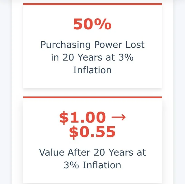
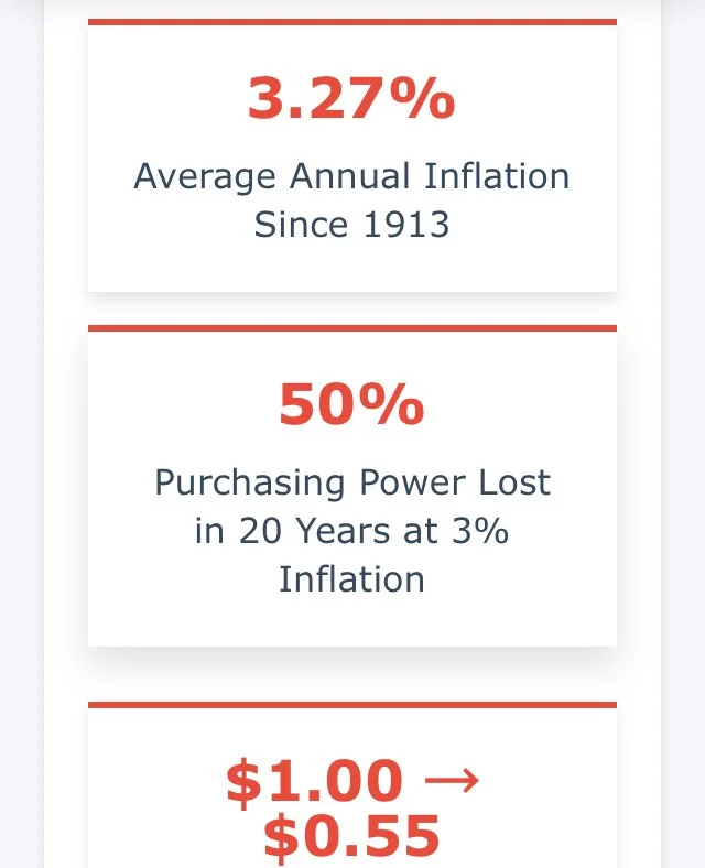
LOSS OF “PURCHASING POWER” OF $1.00 — IMPACTS AT SCALE:
Making policy decisions about HOUSELESSNESS based on outdated DATA or no DATA;
Making policy decisions about “no available” and no “affordable housing” in the community based upon outdated DATA and incomplete DATA; and
Making policy decisions about HOUSED and UNHOUSED populations in the community — whose dollar bills’ values have eroded in purchasing power so significantly — to where paying monthly bills is simply no longer possible.
Where Are We?
These calculations below are made from what is “currently” reported DATA on Wikipedia. HOWEVER, the numbers reported are 25 years old — being based on the 2000 US Census. (NOTE: These are the only Census numbers I have been able to find.) (Note: The latest REVISIONS to the “Demographics” section of WIKIPEDIA’s entry on Laconia — occurred September 1, 2025). It is from that “Demographics” section where the following is taken.) WIKIPEDIA LINK TO LACONIA; REVISIONS LOG history:
The numbers below from Wikipedia include “MEDIAN INCOMES” in Laconia ONLY; however these NUMBERS INCLUDE BOTH renters and property owners combined into the MEDIAN INCOMES listed.
If the MEDIAN INCOMES of “just” RENTERS were reported, the incomes would be lower … and the 30% of those MEDIAN INCOMES would lower what is deduced as “affordable rents”.
The 55 Year Old “30% Rule” for Housing “Rent Affordability” — NEVER Adjusted for Loss of Purchasing Power of a Dollar Bill.
But what is now considered “affordable rent” is based upon a 1969 Rule (i.e., the Brooke Amendment), which initially capped “public” housing rent at 25% of a resident’s income to ensure affordability for low-income households.
This arbitrary threshold was later increased to 30% in 1981, becoming a widely accepted standard for housing affordability. Using outdated (year 2000 Census for Laconia) DATA —currently reported and relied upon in 2025. This Rule was also established in the later 1960’s when, generally speaking, HOUSEHOLDS had one “breadwinner” in the family, and one stay at home parent to nurture, raise and even educate their children. As well, the time frame the rule was created for low income housing by HUD, credit cards were in their infancy and not highly circulated in the American Population. See, Forbes article.
So now, let’s examine the question of “rent affordability”.
WIKIPEDIA reports on Laconia as follows:
The median income for a household in the city was $37,796, and the median income for a family was:
$45,307. [Notice this is not NET INCOME (described below)AND it includes high earner outliers (also described below)].
— Males had a median income of $31,714 versus $22,818 for females.
— The per capita income for the city was $19,540.
— 46.4 % Were HOUSEHOLDS: 30% of $37,796 = $11,338 divided by 12 = $944/month.
— MALE: 30% of $31,714 = $9,514 divided by 12 = $793/month.
— FEMALE: 30% Of $22,818 = $6,845 divided by 12 = $570/month.
— Per capita income for the city was $19,540. 30% Of $19,540 = $5,863 divided by 12 = $488/month.
These calculations DO NOT not include a reduction of income for taxes, utilities, AND DO NOT INCLUDE loss of $1.00 purchasing power (the impact of which is also presented below).
There were 6,724 households, out of which 28.0% had children under the age of 18 living with them, 46.4% were married couples living together, 11.2% had a female householder with no husband present, and 38.0% were non-families.
Impacts at Scale: Loss of Purchasing Power
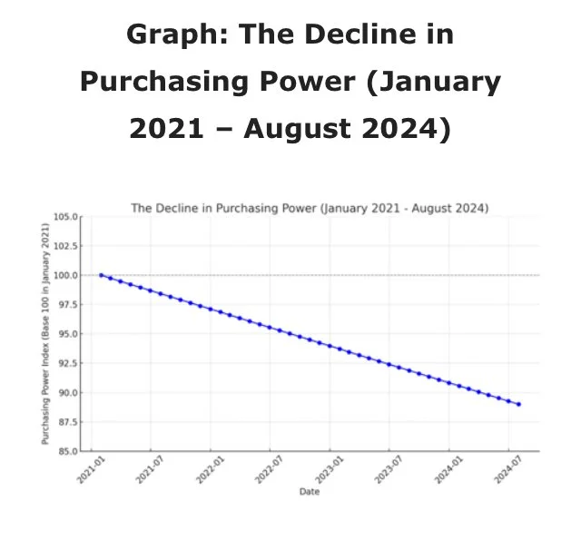
Loss of Purchasing Power of $1.00 by year from 2021-2025
Often declines are reported on a cumulative basis or year-over-year “YOY”. Cumulative declines present an often misleading picture quite different than YOY. SOURCE 1; SOURCE 2:
“Cumulative decline refers to the total decrease in the value of an investment [or purchasing power of $1.00] over a specific period, expressed as a percentage, while year-over-year (YOY) compares the performance of a metric, like revenue [or purchasing power], from one year to the same period in the previous year. Cumulative decline provides a broader view of overall performance, whereas YOY focuses on annual changes.”
At this point in our discussion one can only speculate why policy makers never adjusted the ARBITRARY 30 % RULE and substantially lower it to say 10% or even 5% to account for the significant declines (YOY) in purchasing power of a dollar from 1969-2025.
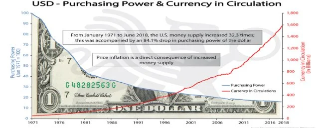
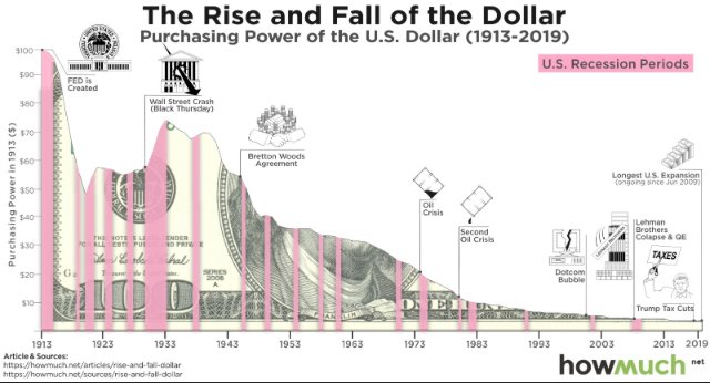
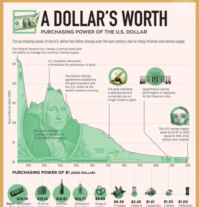
Dollar Bill Purchasing Power Declines 1960-2025 YOY = 800% (1960-2025); 2600% (1920-2025):
1920. $26.14
1960. $8.35
1970. $6.39
1980. $3.50
1990. $2.28
2000. $1.63
2025. $1.00
Given the magnitude this obvious and unabated decline in “purchasing power” of $1.00, one must ask: “Was this purchasing power decline offset by an hourly wage increase over the same time frames?” The charts below indicate the declines were NOT offset. SOURCE CHART BELOW
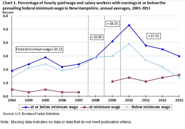

So one must ask, were hourly wages charted above managed and kept “stagnant” by legislative will at federal $5.15/hr and NH $7.25/hr; that is, as the dollar’s purchasing power continued to decrease? YES!
Was and is this intentional? Readers may apply their own Critical Thinking to that question.
“By the end of 2021, the index had dropped to 96, indicating a 4% decline in purchasing power relative to the base year. However, by December 2022, the index stood at 93, signaling a cumulative 7% decline in purchasing power since January 2021.
By mid-2023, the purchasing power index had fallen to 91, with many Americans feeling the pinch as their paychecks stretched less far than they had in previous years. As of August 2024, the purchasing power index has reached 89, marking an 11% decline from the base year. Despite efforts to curb inflation and increase wages, the cumulative effect of the past three years has left many workers struggling to maintain their standard of living.” SOURCE:
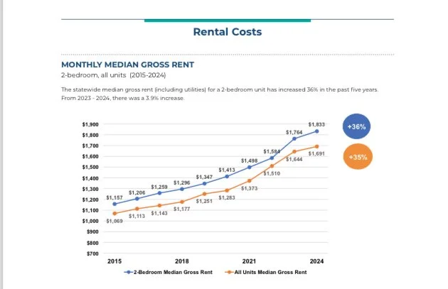
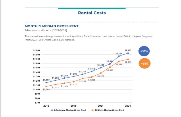
Between 2015-2024 median rents for a 2 BR apartment increased from $1,157 to $1,853. That $1,853 is twice the “affordable rent” for HOUSEHOLDS, 2.5 times the “affordable rent” for males, and 3 times the “affordable rent” for females — as reported above by Wikipedia.
— 46.4 % Were HOUSEHOLDS: 30% of $37,796 = $11,338 divided by 12 = $944/month.
— MALE: 30% of $31,714 = $9,514 divided by 12 = $793/month.
— FEMALE: 30% Of $22,818 = $6,845 divided by 12 = $570/month.
The graph above “The Decline in Purchasing Power January 2021 - August 2024” illustrates the steady decline in purchasing power of those in the Lakes Region. The graph uses 100 as the base value, with each month’s index calculated using the formula outlined above.
The downward trend is stark, highlighting the persistent challenge of balancing wage growth with inflation. Today the average American has a purchasing power that is 11% lower than it was when President Biden took the oath of office.
And that 11% is just over 4 years.
WHAT DOES THIS MEAN IN THE LAKES REGION?
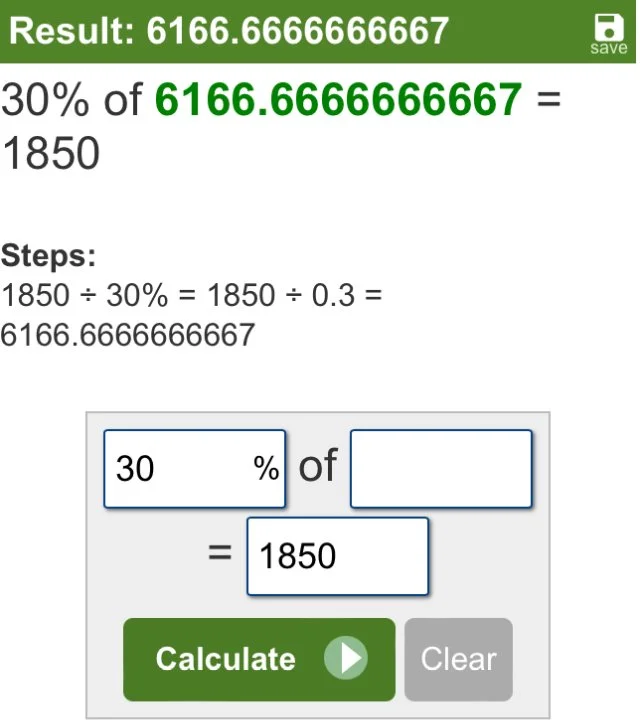
Assuming the $1,853 rent for a 2BR apartment is a realistic average, then applying the 30% threshold of rent to NET INCOME means a HOUSEHOLD must earn $6,166/month ($39.00/hour) to stay within that 1969 30% Rule threshold.
The super-majority of people living in Laconia are not earning $39.00/hr as NET pay, and that does not include utilities and other monthly necessities.

One might reasonably ask who even came up with the 1969 ARBITRARY 30% threshold? IT IS
INDEED “ARBITRARY” AND DATES BACK TO 1969 WHEN ONE BREADWINNER IN A HOUSEHOLD WAS SUFFICIENT.
But why not 5% or even 10% — then or now in 2025?
“Studies reveal that around 40% of middle-income renters are still exceeding the 30% benchmark, and in high-demand metropolitan areas, this number is even higher.”. SOURCE:
“Understanding the 30% Rule. The 30% rule traces its origins back to the 1969 Brooke Amendment, which initially capped public housing rent at 25% of a resident’s income to ensure affordability for low-income households. This threshold was later increased to 30% in 1981, becoming a widely accepted standard for housing affordability. The rule traditionally defines housing costs as including rent or mortgage payments, property taxes, and homeowners insurance. The core intent behind this guideline was to prevent households from becoming “house poor,” a situation where a disproportionate amount of income is consumed by housing, leaving insufficient funds for other necessities like food, transportation, medical care, and savings.
By adhering to this limit, individuals are able to maintain financial balance and pursue other financial goals. The rule serves as a simple benchmark for both renters and homeowners when assessing affordability.
Shifting Economic Landscape
Economic changes have challenged the 30% rule’s universal applicability. Housing costs, including rental and purchase prices, have substantially increased, outpacing wage growth over the past decade. Between 2010 and 2022, home prices rose by 74% while average wages increased by only 54%.” SOURCE
[NOTE: This 54% so-called average wage increases METRIC is inaccurate and misleading. It does not account for the erosion of the value (purchasing power) of each $1.00 on this trend line.
“This disparity means vastly more income is now required for housing in many areas. Student loan debt also presents a challenge, consuming income otherwise available for housing. For instance, a $1,000 increase in student loan debt has correlated with a 1.8% decline in homeownership for recent college graduates under 35 since 2005.
Increased costs for other necessities, like groceries and healthcare, further strain household budgets. These factors make it impractical for many to strictly adhere to the 30% housing guideline.
Key Factors for Housing Affordability
Individual financial considerations influence housing affordability. A person’s income level, after taxes and deductions, directly dictates their capacity to cover housing expenses. Geographic location plays a substantial role, as housing prices vary dramatically across regions. For example, housing in major metropolitan areas often commands a higher percentage of income compared to less populated regions.” SOURCE
December 2024 Report in New Hampshire
This following report is missing crucial data and analyses. As staggering as the numbers are presented in this recent report: “NEW HAMPSHIRE 2024 RESIDENTIAL RENTAL COST SURVEY REPORT” — may appear — it misses Laconia specific data from “unique” local demographics.
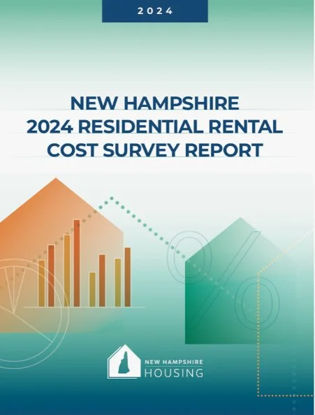
First, the Report is based on median and not mean incomes or NET INCOMES. p. 4
Second, The study is not local to Laconia, which has different demographics than incorporated in the statewide surveys used to produce the charts. It states:
“Information was obtained on 18,512 market-rate rental housing units across the state (12%), and data from 1,809 properties and 7,853 rental units were analyzed using descriptive statistics. An adjustment factor was applied to buildings with more than 10 units to address potential bias towards larger apartment complexes. p. 5
Third, this chart on page 5 is meaningless unless compared against plot lines of both median or mean NET incomes of JUST RENTERS in Laconia AND loss of purchasing power of $1.00 year by year between 2015-2024.
Finally, let’s take at first an example why NET INCOME is important and then look at the effect at scale of high earner “outliers” — ALSO completely overlooked in the report.
EXAMPLE:
“Your net income is equal to your take-home pay after accounting for taxes and other deductions. It is helpful or even vital to know your net income because this is how much of your earnings you actually get to keep.”
“… Calculating average net income involves totaling all incomes across a group, then dividing this combined income figure by the number of people.
For example, consider five individuals with incomes of $30,000, $50,000, $60,000, $70,000 and $100,000. Their total combined income equals $310,000. Dividing this by five people gives an average income of $62,000. Note that in this example, the average of $62,000 exceeds the incomes of three out of the five individuals.
This is due to the outsized impact of the $100,000 outlier high earnings figures. When averages differ markedly from typical incomes, it generally signals that incomes are concentrated among high earners and indicates that financial wellbeing is not broadly shared. …” SOURCE
A Few Concluding Remarks
For purposes of examining the number of “rent burdened” individuals and households in Laconia, ONLY the NET INCOMES of RENTERS is relevant; that is, plotted on a chart (say between 2015 to 2025) and then compared with a plot line of (median or mean) rents, and then a plot line of the loss of purchasing power of $1.00.
Those three plot lines (if overlaid) would reveal a real time assessment of those “rent burdened” in Laconia. Actual utility costs for the same period also plotted and overlaid on the chart would be helpful; if specific to JUST that RENTER population in Laconia.
NET INCOME Outliers in the Laconia demographic including actual home owners; particularly on — say Governors Island, or those owning lake front property with footage on Winnepesauke, Winnisquam, Lakeport, etc. — that is: in any calculation of MEDIAN INCOME of Laconia — (as was the case from the Census records currently appearing on Wikepedia above) — is just poor statistical, and mathematical sampling data. WHY?
Those NET INCOMES in a total population of 16,000+ skew the NET INCOME of that population of RENTERS upward which then skews what is “affordable rent” also upward toward higher earners.
Then for policy making purposes, relevant deductions can be drawn and perhaps discussed.
To be Continued …
For more information on TEAM CONNECTED, please visit our MAIN PAGE.